What will the weather be like tomorrow? How much electrical power can a solar panel produce tomorrow? How much energy will a cooling system consume over the next few days? How many tonnes of cement should I produce today? These are some pertinent questions that industrialists might ask themselves so that they can make the right decisions at the right time. In these situations, forecasting algorithms are a great tool.
But what are they exactly? How can they help us reduce and optimize our energy consumption? How can they be put into practice, more concretely? And how exactly do they relate to Energy Management and Optimization Systems (EMOSs)? In this article, Dorian Grosso and Pascal Lu from METRON’s R&D team answer these questions for us.
What is forecasting exactly?
Most broadly, forecasting is the prediction of future events based on past events. Time series forecasting, more specifically, is the prediction of the future values of a time series based on past observed values. Time series contain a chronological dependency, which means that the current value of the time series depends on past values.
Before forecasting, we usually perform a time series analysis to remove anomalies so that we can extract only meaningful information, such as seasonality and trends. This allows us to make more accurate predictions, which are based on the most valuable data.
The first step of forecasting is to define some operational parameters of the model. These depend on the problem that needs to be solved. Common parameters include:
- The window of inputs (1 hour, 1 day, 1 week …)
- The time horizon of predictions ( 1 hour, 1 day, 1 week …)
- Signal discretization (a point every 1 min, 10 min or 1 hour …)
- The time features (minute of hour, hour of day, day of year)
- Other dynamic features that can influence our forecasts
To forecast the future, we also need information about the past. By analyzing a time series which has taken place over a long period of time, we can identify patterns that happened in the past and predict which ones may occur in the future.
Depending on the case, we may predict the future of the time series using two methods:
- Univariate forecasting: Using only the past of a time series to predict the future of the same time series. For example, we can predict the thermal power of a cooling system based on yesterday’s power.
- Multivariate forecasting: Using other dynamic features that can influence forecasts as well as the same time series. For example, we can predict the electricity production of a solar panel depending on itself and the weather (an external influence).
The next step is to split the time series into a training set and a test set. A training set is used to train an algorithm (estimator) so that it can compute the forecasts. To check the accuracy of the estimator, it must make predictions on a test set. For example, for a time series recorded from 2016 to 2021, we can choose training set data from 2016 to 2020, and test set data for the year 2021. In this case, we can tell if the estimator is accurate if the forecasts are in line with the time series recorded in 2021.
How can we use forecasting in the energy sector?
In the area of energy, examples of time series forecasting include:
- Daily production of electricity of a solar panel, or wind turbine.
- Daily demand (load) of electricity of a factory, building, or house.
- Daily demand of thermal power of a refrigeration system in a factory.
- Market electricity price.
Forecasting energy management over a future time horizon
For example, a client connected to the main grid on a variable energy contract, with a controllable battery and solar panels, must satisfy an electricity demand. The two sources of uncertainty in the future are the electricity demand (load) and the renewable energy production. In order to avoid a black out while minimizing the total electricity cost over the time horizon, we need to forecast them
What are the benefits of forecasting prediction intervals?
We usually forecast both the mean value and a probability distribution. This is so that we can evaluate the level of uncertainty and assess the spectrum of all possible scenarios in the future.
For example, rather than saying that the electricity production of solar panels will be 150 kWh tomorrow, it is better to make a prediction of the probability. If we say that there is a probability of 95% that the electricity production will be between 120 kWh and 180 kWh, we can be aware of the extreme values, such as in the case of high or low production.
Knowing the probability distribution allows the client to
- weigh the risks
- make the best decisions
- minimize the average operation cost
Forecasting prediction intervals allow us to quantify uncertainties from both:
- data noise variance: the training set that we use to train the model is composed of just a few samples.
- model uncertainty: how well the learnt model can approximate the exact model.
There are different strategies to estimate intervals such as:
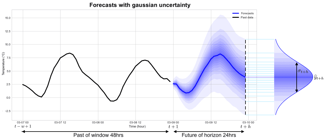
1) Estimating the variance under the hypothesis of Gaussian uncertainty. The error associated with the prediction is represented by a Gaussian distribution characterized by 2 parameters: the average value of the prediction and the standard deviation (square root of the variance). The probability of finding the signal within the interval +/- 2 times the standard deviation around the mean is equal to 95%. The curve on the far right in the figure below represents the predicted probability density for time t+h in the future.
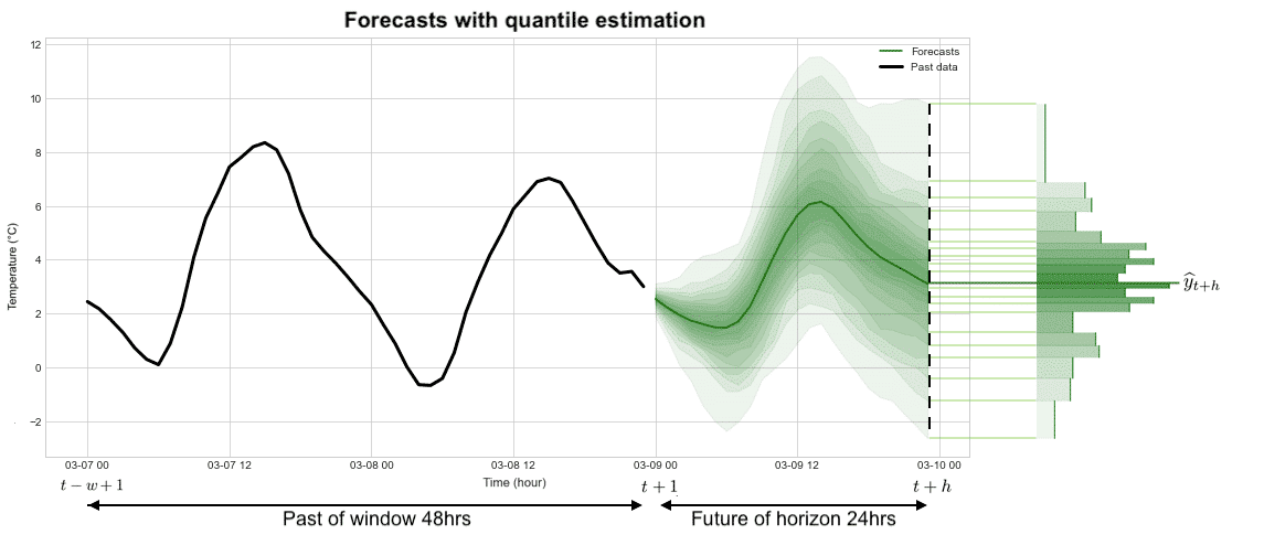
2) Estimating quantiles of the probability distribution under a quantile loss. In this case, we do not assume that the error associated with the prediction is represented by a Gaussian distribution. We do not make assumptions about the shape of the error distribution, we predict the set of quantiles that will characterize the statistical distribution associated with the error. The curve on the far right in the figure below represents the histogram of the predicted probability density for time t+h in the future.
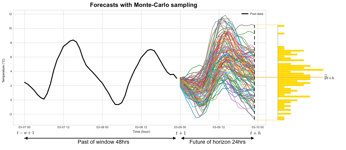
3) Estimating quantiles from an ensemble of future drawn trajectories (Monte Carlo methods). As before, in this case, we do not make any assumptions about the shape of the error distribution, we compute a posteriori the set of quantiles from a large number of plausible trajectories in the future. The curve on the far right in the figure below represents the histogram of the predicted probability density for time t+h in the future.
Forecasting Algorithm Use Case: DeepAR
DeepAR is an autoregressive recurrent neural network algorithm developed by Amazon Research in 2017, where the current observation is reinjected into the neural network to predict the next observation.
For example, DeepAR can be used to predict the amount of thermal power that will be needed for frozen water for a refrigeration system in a factory. For the time series, we define a window (past information) of 48 hours and a horizon (future predictions) over 24 hours. Once the DeepAR is trained, we are able to sample future trajectories given a past signal. From these trajectories, we compute the mean trajectory and several quantiles to quantify the uncertainty. As seen on the figure, the more we sample, the more accurate the mean trajectory and quantiles become.
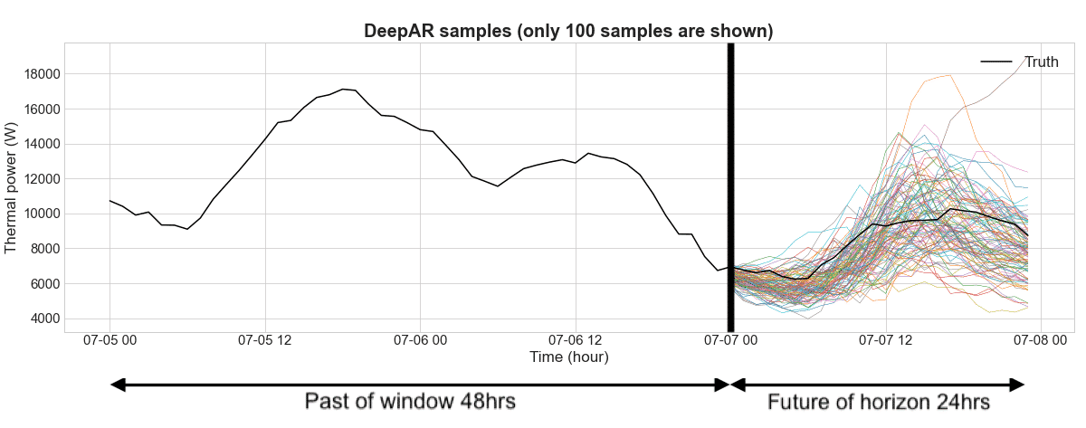
Figure 1: Forecasts for thermal power using frozen water for a refrigerated system where the past window is 48 hrs and the future is of horizon 24 hrs. This graph shows the past time series and 100 future trajectories generated by the DeepAR.
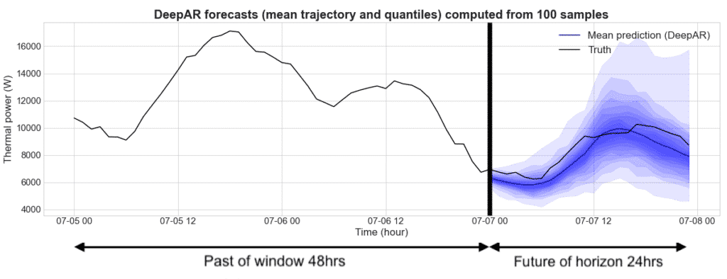
Figure 2: As before, this shows the forecasts for a thermal power using frozen water for a refrigerated system where the past window is 48 hrs and the future is of horizon 24 hrs. However, this graph shows the overall mean trajectory and quantiles computed from 100 future trajectories.
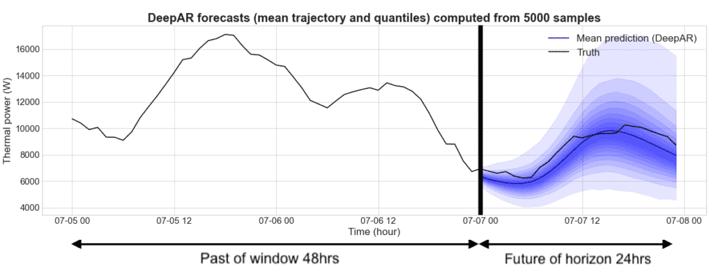
Figure 3: Forecasts for a thermal power using frozen water for a refrigerated system where the past window is 48 hrs and the future is of horizon 24 hrs. This graph represents the mean trajectory and quantiles computed from 5000 sampled future trajectories. Drawing more trajectories helps to smooth quantile curves. This shows us that using more trajectories makes the prediction more precise and accurate.
Key Takeaways
Forecasting algorithms are an intelligent tool that can help us reduce and optimize our energy consumption. These can be used as part of an Energy Management and Optimization system to help make better and more informed decisions, as well as enable teams to be more efficient. Of course, these tools are not here to replace humans, they are here to make us more advanced!
Want to learn more about the METRON Energy Management & Optimization System (EMOS)?

